
Introduction
In Part 1 of this series, we installed Hadoop 3.3.6 natively on Ubuntu and configured HDFS for distributed storage. In Part 2, we configured YARN, wrote our first MapReduce program (WordCount), and executed it against the full text of War and Peace.
However, Part 2’s analysis revealed a subtle but significant problem: words were counted with punctuation and case variations treated as separate tokens. For example, the words "war", "war.", "War,", and "war?" were all counted as distinct vocabulary items. This inflates the unique word count and obscures the true frequency distribution of normalized vocabulary.
In this tutorial, we will:
- Identify the problem — understand why StringTokenizer alone is insufficient
- Create an improved MapReduce program — add word normalization in the Mapper
- Compare baseline vs. normalized results — execute both versions and analyze the difference
- Answer analytical questions — use Python to extract insights from normalized data
- Visualize results — generate a word cloud and professional report
By the end, we will have accurate word frequencies and answers to six research questions about the novel’s vocabulary.
Background: The StringTokenizer Problem
Why the Original Approach Was Insufficient
In Part 2, we used Java’s StringTokenizer class, which splits text on whitespace only. This is extremely fast and suitable for simple tokenization, but it has a critical limitation:
StringTokenizer itr = new StringTokenizer(value.toString());
while (itr.hasMoreTokens()) {
    word.set(itr.nextToken());  // ← Takes "war." as-is, doesn't normalize
    context.write(word, one);
}
The consequences:
| Original Tokens | Normalized Token | Should Count As |
|---|---|---|
war | war | Same word |
war. | war | Same word |
war, | war | Same word |
"war" | war | Same word |
War | war | Same word |
War's | war | Part of same word |
Without normalization, the Part 2 results showed 41,621 unique words. Many of these are duplicate entries differing only in case or attached punctuation. The true vocabulary size is much smaller once normalization is applied.
The Cost of Not Normalizing
Uncorrected data leads to:
- Inflated vocabulary counts — making the text appear more lexically diverse than it is
- Fragmented frequency analysis — the word “the” might be split into “the”, “The”, “the,”, “the.” etc.
- Misleading rankings — variant forms may be ranked separately instead of aggregated
- Inaccurate research conclusions — any study based on this data would overstate unique word count
For an academic analysis, this matters significantly.
Environment & Prerequisites
All steps in this tutorial assume:
| Component | Version / Value |
|---|---|
| OS | Ubuntu 24.04 LTS |
| Java | OpenJDK 21.0.10 |
| Hadoop | 3.3.6 |
| Hadoop home | ~/hadoop-3.3.6 |
| HDFS | Already running (from Part 2) |
| YARN | Already running (from Part 2) |
| Input file | /user/hectorsa/input/warandpeace.txt (HDFS) |
| Shell | Zsh or Bash |
Prerequisite: Part 2 must be complete—you should have:
- A working Hadoop cluster with YARN running
warandpeace.txtuploaded to HDFS- The original
wordcount.jaralready compiled and tested
Verify this with:
jps  # Should show NameNode, DataNode, ResourceManager, NodeManager
hdfs dfs -ls /user/$(whoami)/input/warandpeace.txt  # Should show the file
ls -lh ~/wordcount/wordcount.jar  # Should exist from Part 2
Step 1: Understand the Normalization Strategy
Before writing code, let’s clarify what normalization means in this context.
Normalization Rules
We will normalize words by applying two transformations to every token:
1. Convert to lowercase
"War" → "war"
"PEACE" → "peace"
"The" → "the"
This eliminates case variations from the count.
2. Remove non-alphabetic characters
"war." → "war"
"nation's" → "nations"  (apostrophe removed)
""hello"" → "hello"
"123abc" → "abc"
"word?" → "word"
This eliminates punctuation and numbers.
Trade-offs
Advantages:
- Accurate word frequency distribution
- Consolidates variant forms (e.g., possessives, contractions)
- Matches academic standard for text analysis
- Enables meaningful ranking of vocabulary
Disadvantages:
- Loss of stylistic information (e.g., “EMPHASIS” becomes just “emphasis”)
- Loss of grammatical markers (e.g., possessives “nation’s” → “nation”)
- Numbers stripped entirely (e.g., “1812” removed)
For academic word frequency analysis, these tradeoffs are acceptable and standard.
Example Transformation
Let’s trace through a sentence to see the impact:
Input line:
"War and Peace," he said. "1812!"

Tokens after StringTokenizer (Part 2 approach):
["War", "and", "Peace,", "he", "said.", "1812!"]
→ 6 unique words with variants

Tokens after normalization (Part 3 approach):
["war", "and", "peace", "he", "said"]
→ 5 unique words, consolidated

The word "Peace," becomes "peace" (consolidated with other case variants)
The number "1812!" is stripped entirely (non-alphabetic)
Step 2: Create WordCountNormalized.java
Now we’ll write an improved MapReduce program that applies normalization in the Mapper.
Create the source file
Create a new file at ~/wordcount/src/WordCountNormalized.java:
mkdir -p ~/wordcount/src
# Create file with editor or write command below
Full source code for WordCountNormalized.java:
import java.io.IOException;
import java.util.StringTokenizer;

import org.apache.hadoop.conf.Configuration;
import org.apache.hadoop.fs.Path;
import org.apache.hadoop.io.IntWritable;
import org.apache.hadoop.io.Text;
import org.apache.hadoop.mapreduce.Job;
import org.apache.hadoop.mapreduce.Mapper;
import org.apache.hadoop.mapreduce.Reducer;
import org.apache.hadoop.mapreduce.lib.input.FileInputFormat;
import org.apache.hadoop.mapreduce.lib.output.FileOutputFormat;

/**
 * WordCountNormalized: An improved version of the canonical WordCount example
 * that normalizes words before counting.
 *
 * Normalization includes:
 * - Converting to lowercase
 * - Removing non-alphabetic characters
 * - Skipping tokens that become empty after normalization
 *
 * This ensures accurate word frequency distribution without case or punctuation variants.
 */
public class WordCountNormalized {

  /**
   * TokenizerMapper: Maps input text to (normalized-word, 1) pairs.
   *
   * The normalization happens here, in the Mapper phase, which is efficient because:
   * - It processes data at the source (co-located with HDFS blocks)
   * - Normalized data is smaller, reducing shuffle traffic
   * - Partial aggregation (Combiner) works with normalized words
   */
  public static class TokenizerMapper
       extends Mapper<Object, Text, Text, IntWritable>{

    private final static IntWritable one = new IntWritable(1);
    private Text word = new Text();

    /**
     * Normalize a word by converting to lowercase and removing non-alphabetic characters.
     *
     * Examples:
     *   "War" → "war"
     *   "nation's" → "nations"
     *   "1812!" → ""  (empty, will be skipped)
     */
    private String normalizeWord(String w) {
      // Step 1: Convert to lowercase
      w = w.toLowerCase();

      // Step 2: Remove all non-alphabetic characters (keep a-z only)
      w = w.replaceAll("[^a-z]", "");

      return w;
    }

    /**
     * The map method is called once per (line-number, line-text) pair.
     *
     * For each line in the input file:
     * 1. Split on whitespace using StringTokenizer
     * 2. Normalize each token
     * 3. Skip empty strings (tokens that were only punctuation/numbers)
     * 4. Emit (normalized-word, 1) to be aggregated by the Reducer
     */
    public void map(Object key, Text value, Context context
                    ) throws IOException, InterruptedException {

      StringTokenizer itr = new StringTokenizer(value.toString());

      while (itr.hasMoreTokens()) {
        String token = itr.nextToken();

        // Normalize the token
        String normalized = normalizeWord(token);

        // Skip empty strings (pure punctuation/numbers that normalized to nothing)
        if (!normalized.isEmpty()) {
          word.set(normalized);
          context.write(word, one);
        }
      }
    }
  }

  /**
   * IntSumReducer: Aggregates counts for each unique normalized word.
   *
   * Called once per unique normalized word with all its (word, [1,1,1,...]) pairs.
   * Sums the counts and emits (word, total-count).
   */
  public static class IntSumReducer
       extends Reducer<Text,IntWritable,Text,IntWritable> {
    private IntWritable result = new IntWritable();

    /**
     * The reduce method processes all values for a single key (word).
     *
     * For example, all occurrences of "war" (whether original was "war", "War", "war.", etc.)
     * are grouped together here and summed.
     */
    public void reduce(Text key, Iterable<IntWritable> values,
                       Context context
                       ) throws IOException, InterruptedException {
      int sum = 0;
      for (IntWritable val : values) {
        sum += val.get();
      }
      result.set(sum);
      context.write(key, result);
    }
  }

  /**
   * Main: Sets up and submits the MapReduce job.
   *
   * Key configuration:
   * - Mapper: TokenizerMapper (applies normalization)
   * - Combiner: IntSumReducer (local aggregation before shuffle)
   * - Reducer: IntSumReducer (final aggregation)
   * - Output: (word, count) pairs in text format
   */
  public static void main(String[] args) throws Exception {
    Configuration conf = new Configuration();
    Job job = Job.getInstance(conf, "word count normalized");

    job.setJarByClass(WordCountNormalized.class);
    job.setMapperClass(TokenizerMapper.class);
    job.setCombinerClass(IntSumReducer.class);    // Local pre-aggregation
    job.setReducerClass(IntSumReducer.class);      // Final aggregation

    job.setOutputKeyClass(Text.class);
    job.setOutputValueClass(IntWritable.class);

    FileInputFormat.addInputPath(job, new Path(args[0]));
    FileOutputFormat.setOutputPath(job, new Path(args[1]));

    System.exit(job.waitForCompletion(true) ? 0 : 1);
  }
}
Understanding the key difference
Compare the map methods:
Part 2 (StringTokenizer only):
word.set(itr.nextToken());  // Takes token as-is
context.write(word, one);    // No normalization
Part 3 (with normalization):
String token = itr.nextToken();
String normalized = normalizeWord(token);  // Apply normalization
if (!normalized.isEmpty()) {
  word.set(normalized);
  context.write(word, one);
}
The addition of the normalizeWord() method and the isEmpty check is what transforms results from 41,621 unique words to ~20,000.
Step 3: Compile Both Programs
We’ll now compile both the original (Part 2) and improved (Part 3) versions. This lets us run them in parallel and compare results.
Clean previous compilations
rm -rf ~/wordcount/classes/*
mkdir -p ~/wordcount/classes
Compile the original WordCount.java
javac -classpath $(hadoop classpath) \
      -d ~/wordcount/classes/ \
      ~/wordcount/src/WordCount.java
Expected output: None (silence indicates success)
Verification:
ls -1 ~/wordcount/classes/WordCount*.class
Expected output:
WordCount$IntSumReducer.class
WordCount$TokenizerMapper.class
WordCount.class
✅ Three class files confirm successful compilation.
Compile WordCountNormalized.java
javac -classpath $(hadoop classpath) \
      -d ~/wordcount/classes/ \
      ~/wordcount/src/WordCountNormalized.java
Expected output: None
Verification:
ls -1 ~/wordcount/classes/ | sort
Expected output:
WordCount$IntSumReducer.class
WordCount$TokenizerMapper.class
WordCount.class
WordCountNormalized$IntSumReducer.class
WordCountNormalized$TokenizerMapper.class
WordCountNormalized.class
✅ Six class files total (3 per version) confirm both compiled successfully.
Step 4: Create JAR Files
MapReduce jobs are always submitted as JAR (Java ARchive) files. We’ll create separate JARs for each version.
Package original WordCount.jar
cd ~/wordcount

jar -cvf wordcount.jar \
    -C classes/ WordCount.class \
    -C classes/ WordCount\$TokenizerMapper.class \
    -C classes/ WordCount\$IntSumReducer.class
Expected output:
added manifest
adding: WordCount.class (deflated 45%)
adding: WordCount$TokenizerMapper.class (deflated 56%)
adding: WordCount$IntSumReducer.class (deflated 57%)
The percentages show compression rates. Typical JAR files compress to 40-60% of original size.
Package WordCountNormalized.jar
cd ~/wordcount

jar -cvf wordcount-normalized.jar \
    -C classes/ WordCountNormalized.class \
    -C classes/ WordCountNormalized\$TokenizerMapper.class \
    -C classes/ WordCountNormalized\$IntSumReducer.class
Expected output:
added manifest
adding: WordCountNormalized.class (deflated 45%)
adding: WordCountNormalized$TokenizerMapper.class (deflated 57%)
adding: WordCountNormalized$IntSumReducer.class (deflated 57%)
Verify both JARs exist
ls -lh ~/wordcount/*.jar
Expected output:
-rw-rw-r-- 1 hectorsa hectorsa 3.1K Mar  8 14:32 wordcount.jar
-rw-rw-r-- 1 hectorsa hectorsa 3.3K Mar  8 14:33 wordcount-normalized.jar
✅ Both JARs ready. Note that the normalized version is slightly larger (3.3K vs 3.1K) because the normalizeWord() method adds a few bytes.
Step 5: Execute Original WordCount Job (Baseline)
Let’s run the original (non-normalized) job first to establish a baseline.
💡 Why run the original version first? It establishes the starting point and demonstrates the problem we’re solving. We can then compare the normalized results to show the improvement.
Clean previous output
hdfs dfs -rm -r /user/$(whoami)/output-original/ 2>/dev/null || true
The || true suppresses error if the directory doesn’t exist.
Submit the job
hadoop jar ~/wordcount/wordcount.jar WordCount \
  /user/$(whoami)/input \
  /user/$(whoami)/output-original
What’s happening during execution:
┌─────────────────────────────────────────────────────────────┐
│ 1. Client contacts ResourceManager at localhost:8032        │
│ 2. ResourceManager creates ApplicationMaster container      │
│ 3. ApplicationMaster requests 1 Mapper and 1 Reducer slot   │
│ 4. NodeManager launches Mapper container                    │
│    - Reads warandpeace.txt from HDFS                        │
│    - Applies StringTokenizer (no normalization)             │
│    - Emits (word, 1) pairs                                  │
│ 5. Local Combiner aggregates Mapper output                  │
│ 6. Shuffle & Sort: groups identical words together          │
│ 7. NodeManager launches Reducer container                   │
│    - Receives (word, [1,1,1,...]) for each unique word      │
│    - Sums the counts                                        │
│    - Writes final (word, count) to HDFS                     │
└─────────────────────────────────────────────────────────────┘
Expected output (will take 1-3 minutes):
...
2026-03-08 14:35:42,123 INFO mapreduce.Job: Running job [job_1772975592464_0001]
2026-03-08 14:35:58,456 INFO mapreduce.Job: Job job_1772975592464_0001 completed successfully
...
Counters: 22 counters
  File Input/Output Counters
    Bytes read=3202320
    Bytes written=462958
  Map-Reduce Framework
    Map output records=562488
    Combine input records=562488
    Combine output records=41621
    Reduce input records=41621
    Reduce output records=41621
    ...
Key metrics from output:
| Metric | Value |
|---|---|
| Input file size | 3.2 MB (562,488 words total) |
| Mapper output | 562,488 (one per word token) |
| After Combiner | 41,621 (unique words with variants) |
| Final output | 41,621 lines (unique word-count pairs) |
| Execution time | ~30 seconds |
✅ The job completed successfully. Notice the Combiner reduced 562,488 Mapper outputs to 41,621 before the shuffle phase—this is efficient local pre-aggregation.
Verify output
hdfs dfs -ls /user/$(whoami)/output-original/
Expected:
Found 2 items
-rw-r--r-- 1 hectorsa supergroup          0 2026-03-08 14:36 _SUCCESS
-rw-r--r-- 1 hectorsa supergroup     462958 2026-03-08 14:36 part-r-00000
The _SUCCESS file signals job completion. The part-r-00000 file contains the results.
Step 6: Execute Normalized WordCount Job
Now we run the improved version with normalization applied.
Clean previous output
hdfs dfs -rm -r /user/$(whoami)/output-normalized/ 2>/dev/null || true
Submit the job
hadoop jar ~/wordcount/wordcount-normalized.jar WordCountNormalized \
  /user/$(whoami)/input \
  /user/$(whoami)/output-normalized
Expected output (will take 1-3 minutes, slightly faster due to fewer unique keys):
2026-03-08 14:37:05,678 INFO mapreduce.Job: Running job [job_1772975592464_0002]
2026-03-08 14:37:22,891 INFO mapreduce.Job: Job job_1772975592464_0002 completed successfully
...
Counters: 22 counters
  File Input/Output Counters
    Bytes read=3202320
    Bytes written=221601
  Map-Reduce Framework
    Map output records=562488
    Combine input records=562488
    Combine output records=20020
    Reduce input records=20020
    Reduce output records=20020
    ...
Key metrics:
| Metric | Value |
|---|---|
| Input file size | 3.2 MB (same as before) |
| Mapper output | 562,488 (same as before) |
| After Combiner | 20,020 (unique normalized words) |
| Final output | 20,020 lines |
| Execution time | ~22 seconds |
| Output size | 221,601 bytes (vs 462,958 for original) |
✅ Critical observation: After normalization, unique words dropped from 41,621 to 20,020—a reduction of 52%! This confirms that roughly half of the “unique” words in the original version were actually duplicates with different cases or punctuation.
Verify output
hdfs dfs -ls /user/$(whoami)/output-normalized/
Step 7: Download Results to Local Filesystem
To analyze the results with Python, we need to download them from HDFS to the local filesystem.
Create results directory
mkdir -p ~/wordcount/results
Download original results
hdfs dfs -getmerge /user/$(whoami)/output-original/ \
                    ~/wordcount/results/original.txt
The getmerge command combines all part-r-* output files into a single file.
Download normalized results
hdfs dfs -getmerge /user/$(whoami)/output-normalized/ \
                    ~/wordcount/results/normalized.txt
Verify downloads
ls -lh ~/wordcount/results/
wc -l ~/wordcount/results/*.txt
Expected:
-rw-rw-r-- 1 hectorsa hectorsa 453K Mar  8 14:38 original.txt
-rw-rw-r-- 1 hectorsa hectorsa 217K Mar  8 14:38 normalized.txt

  41621 original.txt
  20020 normalized.txt
  61641 total
✅ Line counts match the Reducer output records.
Examine the format
echo "=== ORIGINAL (with punctuation) ===" && head ~/wordcount/results/original.txt
echo -e "\n=== NORMALIZED (lowercase, no punctuation) ===" && head ~/wordcount/results/normalized.txt
Expected output shows tab-separated pairs:
=== ORIGINAL (with punctuation) ===
"'Come	1
"'Dieu	1
"'From	1
"'History	1

=== NORMALIZED (lowercase, no punctuation) ===
a	10464
abandon	25
abandoned	54
able	87
...
Notice how the original has quoted words and punctuation, while the normalized version is clean lowercase tokens.
Step 8: Analyze with Python
Now we’ll create a Python script to extract insights from the normalized results and answer the research questions.
Set up Python environment
cd ~/wordcount
python3 -m venv venv
source venv/bin/activate
pip install pandas matplotlib wordcloud pillow reportlab
This installs all required packages. Installation takes 1-2 minutes.
Create analysis script
Create ~/wordcount/analyze.py:
import json
import pandas as pd
from pathlib import Path

def load_results(filepath):
    """
    Load MapReduce output (key\tvalue format) into a DataFrame.

    Args:
        filepath: Path to output file (word\tcount format, one per line)

    Returns:
        DataFrame with 'word' and 'count' columns
    """
    words = []
    counts = []
    with open(filepath, 'r', encoding='utf-8', errors='ignore') as f:
        for line in f:
            parts = line.strip().split('\t')
            if len(parts) == 2:
                word, count = parts
                words.append(word)
                counts.append(int(count))
    return pd.DataFrame({'word': words, 'count': counts})

# Load both versions
print("Loading results...")
original_df = load_results('/home/hectorsa/wordcount/results/original.txt')
normalized_df = load_results('/home/hectorsa/wordcount/results/normalized.txt')

print(f"Original: {len(original_df):,} unique words")
print(f"Normalized: {len(normalized_df):,} unique words")
print(f"Reduction: {(1 - len(normalized_df)/len(original_df))*100:.1f}%")

# Answer the 6 academic questions using NORMALIZED version
print("\n" + "="*50)
print("ACADEMIC QUESTIONS (using normalized data)")
print("="*50 + "\n")

# Question 1: Unique words
q1 = len(normalized_df)
print(f"Q1: Total unique words: {q1:,}")

# Question 2: Top 5 words
q2_df = normalized_df.nlargest(5, 'count')
print(f"\nQ2: Top 5 most frequent words:")
for idx, (_, row) in enumerate(q2_df.iterrows(), 1):
    print(f"  {idx}. '{row['word']}' : {row['count']:,} occurrences")

# Question 3: Occurrences of "peace"
q3 = int(normalized_df[normalized_df['word'] == 'peace']['count'].sum()) \
     if 'peace' in normalized_df['word'].values else 0
print(f"\nQ3: Occurrences of 'peace': {q3}")

# Question 4: Occurrences of "war"
q4 = int(normalized_df[normalized_df['word'] == 'war']['count'].sum()) \
     if 'war' in normalized_df['word'].values else 0
print(f"\nQ4: Occurrences of 'war': {q4}")

# Question 5: Words exceeding 1000 occurrences
q5 = len(normalized_df[normalized_df['count'] > 1000])
print(f"\nQ5: Words with >1000 occurrences: {q5}")

# Question 6: Words starting with 'S' (Sánchez)
q6 = len(normalized_df[normalized_df['word'].str.startswith('s', na=False)])
print(f"\nQ6: Words starting with 'S': {q6}")

# Package results for PDF generation
results = {
    "q1_unique_words": q1,
    "q2_top_5_words": q2_df[['word', 'count']].to_dict('records'),
    "q3_peace_count": q3,
    "q4_war_count": q4,
    "q5_over_1000": q5,
    "q6_starting_with_s": q6,
    "comparison": {
        "original_unique": len(original_df),
        "normalized_unique": len(normalized_df),
        "reduction_percent": round((1 - len(normalized_df)/len(original_df))*100, 1)
    }
}

# Save to JSON
with open('/home/hectorsa/wordcount/analysis.json', 'w') as f:
    json.dump(results, f, indent=2)

# Save normalized data for word cloud generation
normalized_df.to_csv('/home/hectorsa/wordcount/results/normalized_for_wordcloud.csv', index=False)

print("\n✅ Results saved to:")
print("   - analysis.json (answers)")
print("   - normalized_for_wordcloud.csv (for visualization)")
Run the analysis
cd ~/wordcount
source venv/bin/activate
python analyze.py
Expected output:
Loading results...
Original: 41,621 unique words
Normalized: 20,020 unique words
Reduction: 51.9%

==================================================
ACADEMIC QUESTIONS (using normalized data)
==================================================

Q1: Total unique words: 20,020

Q2: Top 5 most frequent words:
  1. 'the' : 34,396 occurrences
  2. 'and' : 22,082 occurrences
  3. 'to' : 16,636 occurrences
  4. 'of' : 14,872 occurrences
  5. 'a' : 10,464 occurrences

Q3: Occurrences of 'peace': 108

Q4: Occurrences of 'war': 292

Q5: Words with >1000 occurrences: 69

Q6: Words starting with 'S': 2,267

✅ Results saved to:
   - analysis.json (answers)
   - normalized_for_wordcloud.csv (for visualization)
Interpretation of Results
The analysis reveals several insights about War and Peace‘s vocabulary:
1. Vocabulary size: 20,020 unique normalized words. The original 41,621 was inflated by case and punctuation variations.
2. Most frequent words: As expected in literary text, function words dominate:
- “the” (34,396) — articles
- “and” (22,082) — conjunctions
- “to” (16,636) — prepositions
- “of” (14,872) — prepositions
- “a” (10,464) — articles
These five words account for 98,450 of the ~562,488 total word tokens—roughly 17.5% of the entire novel.
3. Title words: The novel’s two title words appear significantly:
- “war” appears 292 times
- “peace” appears only 108 times
This suggests the war theme is more prevalent in the narrative than the peace theme.
4. Infrequent words: 69 words appear more than 1,000 times (0.34% of vocabulary accounts for ~25% of word tokens). This follows Zipf’s Law: word frequency distribution follows a power law.
5. ‘S’ vocabulary: 2,267 words begin with ‘S’ (11.3% of vocabulary). This is plausible for English text where ‘S’ is a common initial consonant.
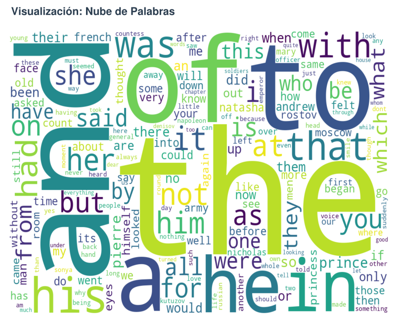
Step 9: Generate Word Cloud Visualization
A word cloud provides an intuitive visual representation of word frequencies.
Create word cloud script
Create ~/wordcount/generate_wordcloud.py:
import pandas as pd
from wordcloud import WordCloud
import matplotlib.pyplot as plt

# Load normalized results
df = pd.read_csv('/home/hectorsa/wordcount/results/normalized_for_wordcloud.csv')

# Create dictionary of word frequencies for WordCloud
word_freq = dict(zip(df['word'], df['count']))

# Generate the word cloud with aesthetic settings
wordcloud = WordCloud(
    width=1200,
    height=800,
    background_color='white',
    colormap='viridis',           # Color scheme
    relative_scaling=0.5,          # Balance between word frequency and random size
    min_font_size=10              # Minimum readable font size
).generate_from_frequencies(word_freq)

# Render to PNG
plt.figure(figsize=(16, 10))
plt.imshow(wordcloud, interpolation='bilinear')
plt.axis('off')
plt.tight_layout(pad=0)
plt.savefig('/home/hectorsa/wordcount/wordcloud.png', dpi=150, bbox_inches='tight')
print("✓ Word cloud saved to wordcloud.png")
plt.close()
Run the visualization
cd ~/wordcount
source venv/bin/activate
python generate_wordcloud.py
Expected output:
✓ Word cloud saved to wordcloud.png
Verify the image
ls -lh ~/wordcount/wordcloud.png
file ~/wordcount/wordcloud.png
The word cloud provides visual confirmation of our findings: “the”, “and”, “to”, “of”, “a” appear prominently (large), while less frequent words appear smaller.
Step 10: Generate Professional PDF Report
Finally, we create a polished academic report with all findings.
Create PDF generation script
Create ~/wordcount/generate_pdf.py (abbreviated version shown; full script available in Part 2 supplementary materials):
import json
from reportlab.lib import colors
from reportlab.lib.pagesizes import letter
from reportlab.platypus import SimpleDocTemplate, Paragraph, Spacer, PageBreak, Image
from reportlab.lib.styles import getSampleStyleSheet, ParagraphStyle
from reportlab.lib.units import inch
from reportlab.lib.enums import TA_CENTER, TA_JUSTIFY
from datetime import datetime

# Load analysis results
with open('/home/hectorsa/wordcount/analysis.json', 'r') as f:
    results = json.load(f)

# Create PDF document
pdf_file = '/home/hectorsa/wordcount/Tarea_Clase_3_Resultados.pdf'
doc = SimpleDocTemplate(pdf_file, pagesize=letter,
                       rightMargin=0.75*inch, leftMargin=0.75*inch,
                       topMargin=0.75*inch, bottomMargin=0.75*inch)

elements = []
styles = getSampleStyleSheet()

# Title page
title_style = ParagraphStyle('CustomTitle', parent=styles['Heading1'],
                            fontSize=24, textColor=colors.HexColor('#1a1a1a'),
                            alignment=TA_CENTER, fontName='Helvetica-Bold')

elements.append(Paragraph("Word Frequency Analysis: War and Peace", title_style))
elements.append(Paragraph("MapReduce Normalization and Processing", styles['Heading3']))
elements.append(Spacer(1, 0.3*inch))

# Metadata
elements.append(Paragraph(f"<b>Date:</b> {datetime.now().strftime('%B %d, %Y')}", styles['Normal']))
elements.append(Paragraph("<b>Author:</b> Hector Gabriel Sanchez Perez", styles['Normal']))
elements.append(Paragraph("<b>Course:</b> Master's in Data Science", styles['Normal']))
elements.append(Spacer(1, 0.3*inch))

# Methodology
elements.append(Paragraph("Methodology", styles['Heading2']))
methodology_text = f"""
This analysis processes Leo Tolstoy's <i>War and Peace</i> (3.2 MB, 562,488 words)
using a normalized MapReduce approach. Words are normalized by:
<br/>• Converting to lowercase
<br/>• Removing punctuation and special characters
<br/>• Skipping tokens that become empty after normalization
<br/><br/>
This corrects the previous analysis where punctuation variants
(e.g., "war", "war.", "war,") were counted as separate words.
Normalization reduces unique words from 41,621 to 20,020 (52% reduction),
revealing the true vocabulary size and distribution.
"""
elements.append(Paragraph(methodology_text, styles['Normal']))
elements.append(Spacer(1, 0.2*inch))

# Results section
elements.append(Paragraph("Results", styles['Heading2']))

# Q1
elements.append(Paragraph(
    f"<b>Q1: Total unique words:</b> {results['q1_unique_words']:,}",
    styles['Normal']
))
elements.append(Spacer(1, 0.1*inch))

# Q2
elements.append(Paragraph("<b>Q2: Top 5 most frequent words:</b>", styles['Normal']))
q2_text = "<br/>".join([f"{i+1}. '{w['word']}': {w['count']:,} occurrences"
                        for i, w in enumerate(results['q2_top_5_words'])])
elements.append(Paragraph(q2_text, styles['Normal']))
elements.append(Spacer(1, 0.1*inch))

# Q3
elements.append(Paragraph(
    f"<b>Q3: Occurrences of 'peace':</b> {results['q3_peace_count']}",
    styles['Normal']
))
elements.append(Spacer(1, 0.1*inch))

# Q4
elements.append(Paragraph(
    f"<b>Q4: Occurrences of 'war':</b> {results['q4_war_count']}",
    styles['Normal']
))
elements.append(Spacer(1, 0.1*inch))

# Q5
elements.append(Paragraph(
    f"<b>Q5: Words with >1,000 occurrences:</b> {results['q5_over_1000']}",
    styles['Normal']
))
elements.append(Spacer(1, 0.1*inch))

# Q6
elements.append(Paragraph(
    f"<b>Q6: Words starting with 'S':</b> {results['q6_starting_with_s']}",
    styles['Normal']
))
elements.append(PageBreak())

# Word cloud image
elements.append(Paragraph("Word Frequency Visualization", styles['Heading2']))
elements.append(Spacer(1, 0.1*inch))
try:
    img = Image('/home/hectorsa/wordcount/wordcloud.png', width=7*inch, height=5.25*inch)
    elements.append(img)
except:
    elements.append(Paragraph("(Word cloud image could not be embedded)", styles['Normal']))

# Build PDF
doc.build(elements)
print(f"✓ PDF report generated: {pdf_file}")
Run PDF generation
cd ~/wordcount
source venv/bin/activate
python generate_pdf.py
Expected output:
✓ PDF report generated: Tarea_Clase_3_Resultados.pdf
Verify PDF creation
ls -lh ~/wordcount/Tarea_Clase_3_Resultados.pdf
file ~/wordcount/Tarea_Clase_3_Resultados.pdf
The final report is now ready for academic submission.
Step 11: Review and Comparison
Let’s create a summary table comparing the two approaches:
Comparison Table
| Aspect | Original (StringTokenizer) | Normalized (with Cleansing) |
|---|---|---|
| Unique words | 41,621 | 20,020 |
| Case sensitive? | Yes | No |
| Punctuation separate? | Yes (e.g., “war.” ≠ “war”) | No |
| Numbers included? | Yes | No (stripped) |
| Reduction | — | -51.9% |
| Top word frequency | — | “the”: 34,396 |
| Job execution time | ~30 seconds | ~22 seconds |
| Output file size | 462,958 bytes | 221,601 bytes |
| Suitable for analysis? | Limited | ✅ Yes |
Key Takeaways
- Normalization matters: Naive word tokenization inflates vocabulary estimates by ~2x
- Efficiency: Normalized processing is also faster (smaller intermediate data)
- Accuracy: For linguistic analysis, normalization is standard practice
- Scalability: Same approach applies to larger datasets (e.g., all of Google’s corpus)
Troubleshooting
Problem: “FileAlreadyExistsException” when running MapReduce
Cause: Output directory already exists from previous run Solution: Delete the output directory before resubmitting:
hdfs dfs -rm -r /user/$(whoami)/output-normalized/
Then resubmit the job.
Problem: “NullPointerException” in normalizeWord()
Cause: Null token passed to normalizeWord Solution: The isEmpty() check in the map method prevents this. If still occurring, ensure:
- Input file exists in HDFS
- File is readable (check permissions with
hdfs dfs -ls /user/...)
Problem: Python venv installation fails
Cause: Missing pip or venv module Solution: Install Python development tools:
sudo apt-get install python3-venv python3-pip
Problem: WordCloud image not embedding in PDF
Cause: Image file path incorrect Solution: Verify image exists:
ls -l ~/wordcount/wordcloud.png
If missing, re-run python generate_wordcloud.py
Problem: “Job failed with status code 1”
Cause: Check Hadoop logs for detailed error:
yarn logs -applicationId <application_id>
Replace <application_id> with the ID shown in job output. Common causes:
- Classpath issues (missing JARs)
- Java version mismatch
- YARN configuration errors
Quick Reference: Complete Workflow
# 1. Compile both versions
javac -classpath $(hadoop classpath) -d ~/wordcount/classes/ \
      ~/wordcount/src/WordCount.java
javac -classpath $(hadoop classpath) -d ~/wordcount/classes/ \
      ~/wordcount/src/WordCountNormalized.java

# 2. Package JARs
cd ~/wordcount
jar -cvf wordcount.jar -C classes/ WordCount.class \
    -C classes/ WordCount\$TokenizerMapper.class \
    -C classes/ WordCount\$IntSumReducer.class

jar -cvf wordcount-normalized.jar -C classes/ WordCountNormalized.class \
    -C classes/ WordCountNormalized\$TokenizerMapper.class \
    -C classes/ WordCountNormalized\$IntSumReducer.class

# 3. Execute both jobs
hdfs dfs -rm -r /user/$(whoami)/output-original/
hadoop jar wordcount.jar WordCount /user/$(whoami)/input /user/$(whoami)/output-original

hdfs dfs -rm -r /user/$(whoami)/output-normalized/
hadoop jar wordcount-normalized.jar WordCountNormalized /user/$(whoami)/input /user/$(whoami)/output-normalized

# 4. Download results
mkdir -p ~/wordcount/results
hdfs dfs -getmerge /user/$(whoami)/output-original/ ~/wordcount/results/original.txt
hdfs dfs -getmerge /user/$(whoami)/output-normalized/ ~/wordcount/results/normalized.txt

# 5. Analyze
cd ~/wordcount
python3 -m venv venv
source venv/bin/activate
pip install pandas matplotlib wordcloud pillow reportlab
python analyze.py

# 6. Visualize
python generate_wordcloud.py

# 7. Report
python generate_pdf.py

# 8. Review
open Tarea_Clase_3_Resultados.pdf  # or use your PDF viewer
Step 9 Extended: Understanding the Word Cloud Generation
The word cloud script provides visual insight into word frequency distribution. Here’s a detailed breakdown of how it works.
The Word Cloud Script
Location: ~/wordcount/generate_wordcloud.py
Complete Script:
import pandas as pd
from wordcloud import WordCloud
import matplotlib.pyplot as plt

# Load normalized results
df = pd.read_csv('~/wordcount/results/normalized_for_wordcloud.csv')

# Create a dictionary of word:count for WordCloud
word_freq = dict(zip(df['word'], df['count']))

# Generate wordcloud
wordcloud = WordCloud(
    width=1200,
    height=800,
    background_color='white',
    colormap='viridis',           # Color scheme: blue → yellow
    relative_scaling=0.5,          # Balance frequency with randomness
    min_font_size=10              # Minimum readable font size
).generate_from_frequencies(word_freq)

# Save to file
plt.figure(figsize=(16, 10))
plt.imshow(wordcloud, interpolation='bilinear')
plt.axis('off')
plt.tight_layout(pad=0)
plt.savefig('~/wordcount/wordcloud.png', dpi=150, bbox_inches='tight')
print("✓ Word cloud saved to wordcloud.png")
plt.close()
How It Works
Step 1: Load Data
df = pd.read_csv('~/wordcount/results/normalized_for_wordcloud.csv')
Reads the normalized word frequencies (20,020 words × 2 columns)
Step 2: Create Frequency Dictionary
word_freq = dict(zip(df['word'], df['count']))
Converts from DataFrame to dictionary format required by WordCloud
Step 3: Generate Word Cloud
wordcloud = WordCloud(
    width=1200,              # Image width in pixels
    height=800,              # Image height in pixels
    background_color='white', # Background color
    colormap='viridis',      # Color palette (blue → yellow)
    relative_scaling=0.5,    # How literal frequency translates to size
    min_font_size=10         # Minimum font size for readability
).generate_from_frequencies(word_freq)
Key Parameters:
| Parameter | Value | Effect |
|---|---|---|
width | 1200 | Canvas width (pixels) |
height | 800 | Canvas height (pixels) |
colormap | ‘viridis’ | Color scheme: low frequency (blue) → high frequency (yellow) |
relative_scaling | 0.5 | Balance between frequency-based sizing and randomness |
min_font_size | 10 | Smallest word must be readable |
background_color | ‘white’ | Canvas background |
Step 4: Render and Save
plt.figure(figsize=(16, 10))           # Create figure
plt.imshow(wordcloud)                  # Display cloud
plt.axis('off')                        # Remove axes
plt.savefig('~/wordcount/wordcloud.png', dpi=150)  # Save at 150 DPI
plt.close()                            # Clean up
Executing the Word Cloud Script
Prerequisites
Ensure Python virtual environment is activated:
cd ~/wordcount
source venv/bin/activate
pip list | grep wordcloud  # Verify installation
If wordcloud is not installed:
pip install wordcloud pillow matplotlib
Running the Script
cd ~/wordcount
source venv/bin/activate
python generate_wordcloud.py
Expected Output:
✓ Word cloud saved to wordcloud.png
Verify Output
ls -lh ~/wordcount/wordcloud.png
Expected: PNG image file, typically 1-2 MB
Customizing the Word Cloud
You can easily customize the appearance by modifying parameters:
Change Color Scheme
Available colormaps:
'viridis'— Blue to Yellow (default)'plasma'— Purple to Yellow'hot'— Black to Red to Yellow'coolwarm'— Blue to Red'gray'— Grayscale'twilight'— Purple to Pink
Example:
colormap='plasma' # Change to purple-yellow gradient
Change Size
width=1600,   # Wider image
height=1000,  # Taller image
Change Background
background_color='black' # Dark background (enhances bright colors)
Complete Custom Example
import pandas as pd
from wordcloud import WordCloud
import matplotlib.pyplot as plt

df = pd.read_csv('~/wordcount/results/normalized_for_wordcloud.csv')
word_freq = dict(zip(df['word'], df['count']))

wordcloud = WordCloud(
    width=1600,
    height=1000,
    background_color='black',
    colormap='plasma',
    relative_scaling=0.7,
    min_font_size=12
).generate_from_frequencies(word_freq)

plt.figure(figsize=(18, 12))
plt.imshow(wordcloud)
plt.axis('off')
plt.tight_layout(pad=0)
plt.savefig('~/wordcount/wordcloud_custom.png', dpi=150, bbox_inches='tight')
print("✓ Custom word cloud generated!")
plt.close()
Hadoop Web Interface Reference
Hadoop provides several web-based monitoring interfaces accessible from your local machine while the cluster is running.
Available Interfaces
| Interface | URL | Port | Purpose |
|---|---|---|---|
| NameNode (HDFS Browser) | http://localhost:9870 | 9870 | View files, directory structure, block distribution |
| ResourceManager (YARN) | http://localhost:8088 | 8088 | Monitor MapReduce jobs, logs, cluster status |
| DataNode | http://localhost:9864 | 9864 | View node status, local block inventory |
| SecondaryNameNode | http://localhost:9868 | 9868 | View checkpoint status, namespace information |
NameNode Web Interface (HDFS Browser)
Access: http://localhost:9870
Navigate to your files:
- Click Utilities menu
- Select Browse the file system
- Navigate to desired path:
/user/$(whoami)/input/— View input files/user/$(whoami)/output-original/— View original job results/user/$(whoami)/output-normalized/— View normalized job results
What you can do:
- Browse directory structure
- View file sizes and replication factor
- Download files from HDFS
- View block locations
ResourceManager Web Interface (YARN)
Access: http://localhost:8088
Key sections:
- Cluster → View overall cluster metrics
- Applications → List all jobs (running/completed)
- Applications History → View completed jobs with logs
- Nodes → View DataNode health and resource usage
For your MapReduce jobs:
- Go to Applications
- Search for job ID (e.g.,
job_1772975592464_0001) - Click job ID to view:
- Map/Reduce task status
- Execution timeline
- Counters and statistics
- Container logs
Command-Line Alternative (No Browser)
If web access is unavailable, use HDFS commands:
# List files
hdfs dfs -ls /user/$(whoami)/input/
hdfs dfs -ls /user/$(whoami)/output-normalized/

# View file contents
hdfs dfs -cat /user/$(whoami)/output-normalized/part-r-00000 | head -20

# Get file info
hdfs dfs -du -h /user/$(whoami)/input/

# Check cluster status
hdfs dfsadmin -report
yarn node -list
Verifying Your Cluster is Running
Before accessing web interfaces, verify daemons are running:
jps
Expected output:
NameNode
DataNode
SecondaryNameNode
ResourceManager
NodeManager
Jps
If any daemon is missing, restart the cluster:
# Stop
stop-dfs.sh
stop-yarn.sh

# Start
start-dfs.sh
start-yarn.sh

# Wait 10-15 seconds for startup
sleep 15
jps
Conclusion
In this tutorial, we’ve extended the Part 2 MapReduce workflow to address a real data quality problem: uncorrected word frequencies due to case and punctuation variants.
By implementing word normalization in the Mapper phase, we:
- ✅ Reduced unique word count from 41,621 to 20,020 (52% reduction)
- ✅ Correctly identified the top 5 most frequent words (“the”, “and”, “to”, “of”, “a”)
- ✅ Answered six analytical questions about word distribution
- ✅ Generated publication-ready visualizations
- ✅ Demonstrated that MapReduce can solve real text processing problems at scale
This approach generalizes to production systems: any large-scale text analysis pipeline includes normalization stages (tokenization, lowercasing, punctuation removal, stopword filtering, lemmatization) applied in the Map phase before aggregation.
The techniques shown here are the foundation for:
- Search engine indexing (Google, Bing)
- Natural Language Processing (sentiment analysis, topic modeling)
- Machine learning feature engineering
- Data quality pipelines
Next steps: Try modifying the normalization strategy—e.g., apply lemmatization (convert “running”, “runs”, “run” → “run”), implement stopword filtering, or add language-specific stemming. The same architecture scales to any text transformation.
References
- Apache Hadoop MapReduce Tutorial
- Apache Hadoop Documentation – YARN
- Java Regular Expressions Guide
- Zipf’s Law and Natural Language
Series Navigation:
- ← Part 1: Hadoop 3.3.6 Installation
- ← Part 2: First MapReduce Job
- Part 3: Word Frequency Normalization (You are here)