
SilverBullet Quick Start Guide for Students: A Practical Workflow for Master Classes
A practical guide to getting productive with SilverBullet for academic work. Based on the official video series by Zef Hemel.
Productivity, Education
A practical guide to getting productive with SilverBullet for academic work. Based on the official video series by Zef Hemel.
I moved from Obsidian to SilverBullet, an open-source web-based note-taking platform. Here is why I made the switch, what I learned, and a complete installation guide based on my real experience getting it running on an ARM server with Cloudflare Access.
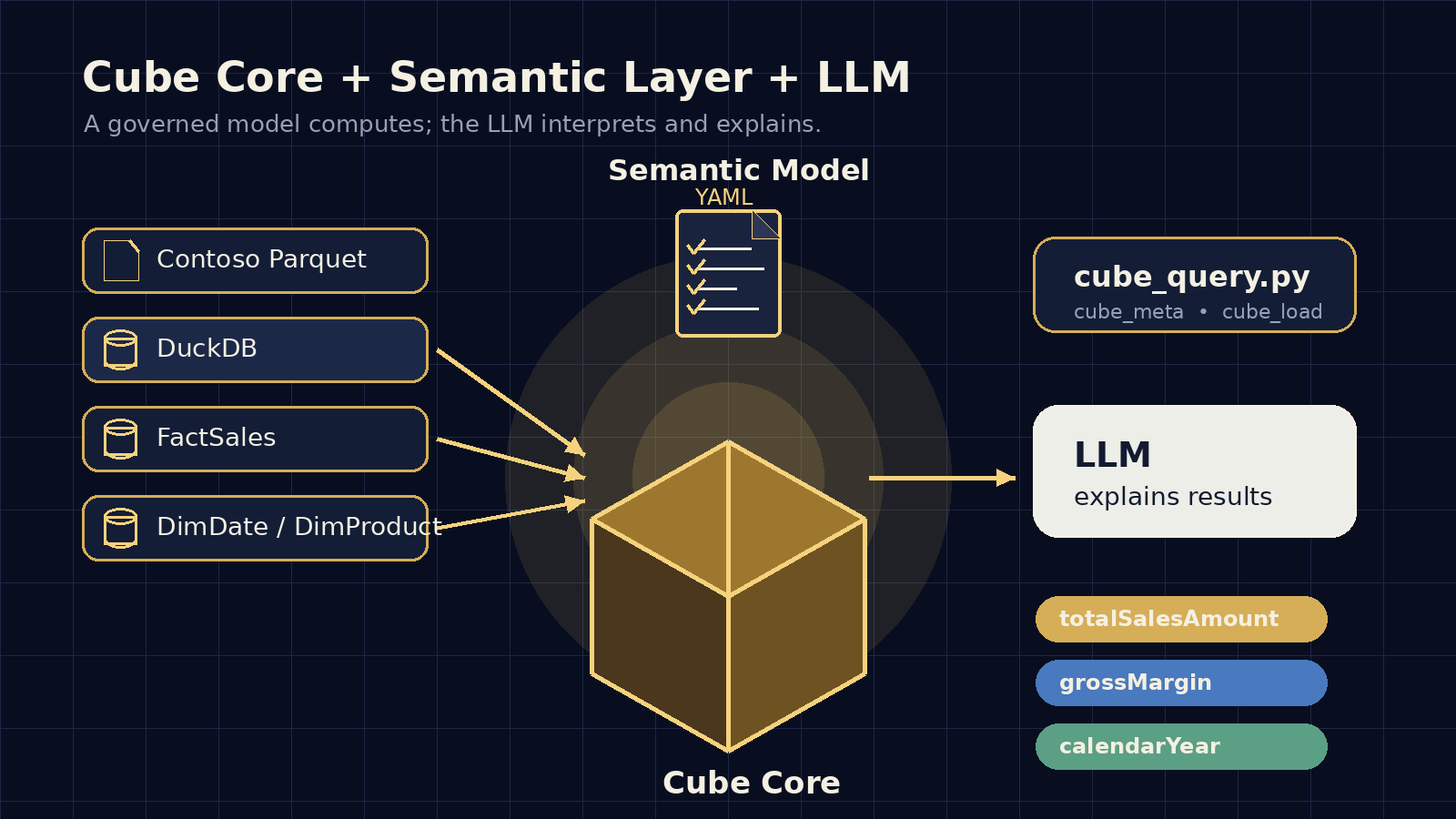
A didactic guide to remember how to build a semantic layer with Cube Core, DuckDB, and Contoso: YAML semantics, Python helper, notebook implementation, and LLM usage for deterministic analytics.

A practical learning workflow inspired by a NotebookLM video: use AI to extract mental models, map expert disagreements, and test real understanding instead of collecting passive summaries.

How I moved CFOCoder from WordPress to Astro, preserved posts and images, kept redirects working, and ended up with a faster, safer static blog.

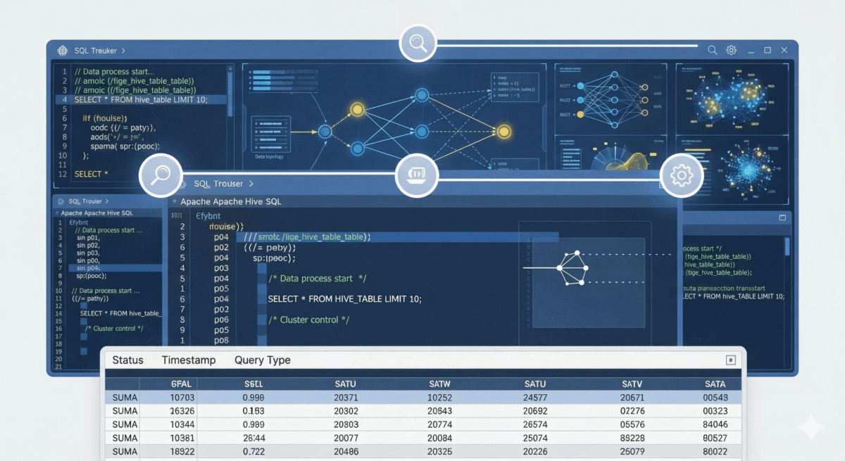
Part 7 in the Hadoop and Hive Tutorial Series
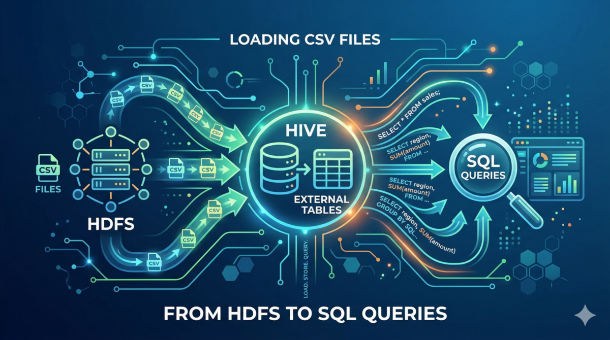
Part 6 in the Hadoop and Hive Tutorial Series
Part 5 in the Hadoop and Hive Tutorial Series