

This is a short quick guide on advanced SQL Server topics, that I recently learned in this course from Udemy. The examples run in this post, use the AdventureWorks2019 sample database provided by Microsoft.
Table of Contents
- Window Functions
- Correlated SubQueries
- PIVOT and UNPIVOT
- Common Table Expressions
- Temporary Tables
- SQL Programming
Window Functions
OVER() Function
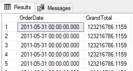
OVER() is a function used after an aggregate function like SUM() to show the same aggregate value repeated on every row. In my opinion, this works similarly to the ALL() function in DAX. It is useful for making calculations at row level, for example, when we want to calculate the % of the grand total
SELECT
OrderDate,
GrandTotal = SUM(TotalDue) OVER()
FROM
AdventureWorks2019.Sales.SalesOrderHeader
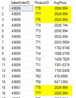
OVER() can use arguments like PARTITION BY and ORDER BY to refine the level of aggregation at row level
SELECT
SalesOrderID,
ProductID,
AvgPrice = AVG(UnitPrice) OVER(PARTITION BY SalesOrderID ORDER BY ProductID DESC)
FROM
Sales.SalesOrderDetail
Ranking of rows
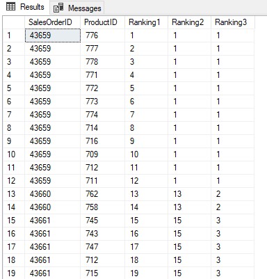
Window functions also allow us to rank rows by using one of the 3 functions alongside the OVER() function:
- ROW_NUMBER(): Returns the sequential rank of each row within the partition. For rows with the same value, it assigns a different rank number regardless if the value is the same.
- RANK(): Returns the rank of each row within the partition. For rows with the same value, it assigns the same ranking number to these, but it skips the ranking number for the next row with a different value, thus leaving gaps in the sequential numbering.
- DENSE_RANK(): Used when we want to rank the rows of a table with no gaps in the ranking numbering. Rows with the same value, also get the same ranking number, but it doesn’t skip the ranking numbering for the next row with a different value.
SELECT
SalesOrderID,
ProductID,
Ranking1 = ROW_NUMBER() OVER(ORDER BY SalesOrderID),
Ranking2 = RANK() OVER(ORDER BY SalesOrderID),
Ranking3 = DENSE_RANK() OVER(ORDER BY SalesOrderID)
FROM
Sales.SalesOrderDetail
LEAD() and LAG()
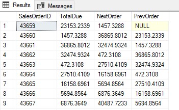
These functions allow us to grab values from subsequent or previous records relative to the position of the current record in the table. These functions are useful when we want to compare a value in a column to the next or previous value side by side in the same row. These functions are similar to the DAX functions NEXT() and PREVIOUS()
SELECT
SalesOrderID,
TotalDue,
NextOrder = LEAD(TotalDue) OVER(ORDER BY SalesOrderID),
PrevOrder = LAG(TotalDue) OVER(ORDER BY SalesOrderID)
FROM
AdventureWorks2019.Sales.SalesOrderHeader
Correlated SubQueries
Subqueries in the SELECT statement
These subqueries, run once for every row in the table and return a scalar value that can come from any other table
SELECT
SalesOrderID,
AverageValue = (SELECT AVG(ListPrice) FROM AdventureWorks2019.Production.Product)
FROM
AdventureWorks2019.Sales.SalesOrderHeader
Subqueries in the WHERE statement (WHERE EXISTS)
These queries are useful when we want to use data from other Tables just as a way to apply criteria in the WHERE statement without having to bring such a field from another table with a JOIN statement.
SELECT
A.SalesOrderID,
A.OrderDate,
A.TotalDue
FROM
AdventureWorks2019.Sales.SalesOrderHeader A
WHERE EXISTS
(
	SELECT
	1
	FROM
	AdventureWorks2019.Sales.SalesOrderDetail B
	WHERE B.LineTotal > 5000
)
PIVOT and UNPIVOT
They work similarly to the Pivot Tables in Excel. Pivot expands criteria from a field as columns, whereas Unpivot does the opposite.
Example of Pivot
This is the starting table called #PivotExample, in this case, we want to pivot the ProductCategoryName as columns for each Category
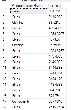
Below is the code to pivot the table above, the fields in the SELECT statement, correspond to each of the columns we want to pivot to. In this case, we are aggregating the field “LineTotal” with a SUM().
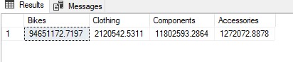
SELECT
B.Bikes,
B.Clothing,
B.Components,
B.Accessories
FROM
#PivotExample A

PIVOT(
	SUM(LineTotal)
	FOR ProductCategoryName IN ([Bikes],[Clothing],[Components], [Accessories])
) B
The end result of the Pivot Table is the following:
Example of Unpivot
To Unpivot the table above, we use the following code. The items in the SELECT statement (Categories and Total) correspond to the fields that are inside the UNPIVOT function, the first one is the name that would aggregate the values from the columns, and the second one, has the list with the name of the columns that would later become the Categories.
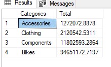
SELECT
Categories = B.Categories,
Total = B.Total
FROM #UnpivotExample A

UNPIVOT
(
 Total FOR Categories IN (Accessories, Clothing, Components, Bikes)
) B
And this is how the result of the code looks like for an Unpivotted Table
Common Table Expressions
Basic CTEs
Useful for making nested queries easier to read, besides the fact that each layer or step can be referenced several times as needed, and the steps have recursivity, as they can refer themselves. Common Table Expressions create a temporary table under the hood for each layer or step, but the steps can only be referenced within the scope of the current query, up until the final SELECT statement.
In the example below, Step1 is referenced in Step2, and in the final SELECT, Step2 is referenced twice, once in the FROM statement (From Step2 A) and a second time in the ON statement to create a new column based on Step2
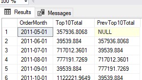
WITH Step1 AS
(
SELECT
OrderDate,
TotalDue,
OrderMonth = DATEFROMPARTS(YEAR(OrderDate),MONTH(OrderDate),1),
OrderRank = ROW_NUMBER() OVER(PARTITION BY DATEFROMPARTS(YEAR(OrderDate),MONTH(OrderDate),1) ORDER BY TotalDue DESC )
FROM
AdventureWorks2019.Sales.SalesOrderHeader
),

Step2 AS
(
SELECT
OrderMonth,
Top10Total = SUM(TotalDue)
FROM
Step1
WHERE OrderRank <= 10
GROUP BY OrderMonth
)

SELECT
A.OrderMonth,
A.Top10Total,
PrevTop10Total = B.Top10Total
FROM Step2 A
LEFT JOIN Step2 B
ON A.OrderMonth = DATEADD(MONTH,1,B.OrderMonth)
ORDER BY 1 ASC
The result of the code above likes like this:
Recursive Common Table Expressions
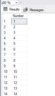
The ability for Common Table Expressions, to call themselves, makes them ideal for generating a series of values. In the example below, we create a consecutive series of integers from 1 to 150. SQL Server limits recursion to 100 iterations, but we can override this limitation with “OPTION(MAXRECURSION 150)“
WITH IntegerSeries AS
(
	SELECT 1 as Number

	UNION ALL

	SELECT
	Number +1
	FROM IntegerSeries
	WHERE Number < 149
)

SELECT
Number
FROM
IntegerSeries
OPTION(MAXRECURSION 150)
This is the result of the code:
Temporary Tables
Temporary Tables work like normal tables, with the difference that their name starts with “#” and they only live for the duration of the current session. Unlike the temporary tables created by Common Table Expressions, Temporary Tables can be referenced anywhere in the code for the current session, can handle large quantities of data, can be optimized, and are easier to debug, so temporary tables are a bit more flexible compared to Common Table Expressions.
Because Temporary Tables don’t disappear after a SELECT statement, they can create issues when running the same code in the same session, as the table already exists, so it is always good to DROP the temporary table after is used.
Create Temporary Tables with SELECT – INTO
This is a short way of creating a temporary table, we don’t need to run the CREATE statement as we do with a normal table. We just have to put the INTO clause before the FROM clause. The name of the temporary table is #TempSales1.
SELECT
SalesOrderID,
Total = SUM(TotalDue)
INTO #TempSales1
FROM
AdventureWorks2019.Sales.SalesOrderHeader
GROUP BY SalesOrderID
Create Temporary Tables with CREATE – INSERT INTO
This is much closer to the traditional way of creating a table, we first create it and then insert rows into it with the result of a SELECT statement. This is a more explicit way of creating temporary tables.
After the CREATE statement, we need to insert “INSERT INTO” before the SELECT statement that contains the information we want to insert into the temporary table.
It is not necessary to indicate the fields we are inserting, but it is better to be explicit and gives us more flexibility in case we want to add extra fields to the temporary table.
CREATE TABLE #TempSales3
(
	SalesOrderID INT,
	Total MONEY
)

INSERT INTO #TempSales3
(
SalesOrderID,
Total
)

SELECT
SalesOrderID,
Total = SUM(TotalDue)
FROM
AdventureWorks2019.Sales.SalesOrderHeader
GROUP BY SalesOrderID
Update Tables with a conditional CASE statement
UPDATE #SalesOrders
SET
TaxFreightBucket =
  CASE
    WHEN TaxFreightPercent < 0.1 THEN 'Small'
    WHEN TaxFreightPercent < 0.2 THEN 'Medium'
    ELSE 'Large'
  END
Update certain records of Table (UPDATE – SET – WHERE)
UPDATE #SalesOrders
SET OrderCategory = 'Holiday'
WHERE DATEPART(QUARTER,OrderDate) = 4
Update Tables based on values on another table (UPDATE – SET – FROM-JOIN)
This is a way to update a table based on the values coming from another table:
UPDATE #ProductsSold2012
SET ProductName = b.Name
FROM AdventureWorks2019 A
JOIN AdventureWorks2019.Production.Product B
ON A.ProductID = B.ProductID
Table Indexes
Indexes are objects of a database that help run the queries faster. There are two types of Indexes, clustered and Non-Clustered.
There can only be one Clustered Index on a table. A Primary Key is an example of a clustered index. Clustered Indexes are usually assigned to columns that uniquely identify the records of a table. We should apply a Clustered Index to fields of a table that are most likely to be used in a JOIN against another table.
A Table can have several Non-Clustered Indexes, and we apply them to fields that would be joined to fields in other tables besides the ones already covered by Clustered Indexes.
The idea is to add a Clustered Index first, and then add Non-Clustered Indexes as needed to cover additional fields used in JOINs against our table.
We typically add indexes after the data has been inserted into the table as it takes longer to insert data once indexes have been added.
To create an index, either Clustered or Non-Clustered, we can add one of these lines of code after we have inserted data into the table.
CREATE CLUSTERED INDEX  Sales_idx ON #SalesTable(SalesOrderID)

CREATE NONCLUSTERED INDEX Sales_idx2 ON #ProductsTable(ProductID)
SQL Programming
Variables
We create variables with the DECLARE statement and the “@” sign preceding the variable word and the type of value, followed by the SET statement and the initial value that we are assigning to the variable. Later when we call the variable, we can get the value of the variable by using the SELECT statement followed by the variable name, including the “@” sign.
Variables can hold scalar values such as numbers, text, or dates.
DECLARE @MyValue INT
SET @MyValue = 74


SELECT @MyValue AS Header1
DECLARE @AvgPrice MONEY
SET @AvgPrice =
(
SELECT
AvgPrice = SUM(TotalDue)
FROM
AdventureWorks2019.Sales.SalesOrderHeader
)

SELECT @AvgPrice AS AvgPrice
Functions
Functions are blocks of logic that can be re-used when they get called somewhere in the code. Functions may take arguments or not.
Functions live in the function folder of the Database, so in the example below, we put the word “dbo” followed by a dot and the name of the function. We also need to specify the type of data it returns, in this case, “RETURNS INT”, and inside the chunk of code that is between BEGIN and END, we need to also specify the value that the function returns, in this case, the sum of the two variables
USE AdventureWorks2019
GO


CREATE FUNCTION dbo.ufnMyFunction1 (@Argument1 INT, @Argument2 INT)
RETURNS INT

BEGIN
	RETURN @Argument1 + @Argument2
END
To call a function later in the code, we can call it using the SELECT statement followed by the schema, the function name, and the parenthesis, with or without arguments.
SELECT dbo.ufnMyFunction1(10, 20) AS Result
Stored Procedures
Stored Procedures are database objects that provide the flexibility to execute single or multiple blocks of code that can do anything from database maintenance to running outputs of multiple select statements. Stored Procedures can use parameters like a function, and not necessarily have to return a value like functions.
Procedures are stored inside the Programmability folder of the database.
They are created in a similar way to functions, but since they don’t have to return a value, we don’t include any RETURN statement.
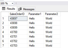
CREATE PROCEDURE dbo.myProcedure1 (@Param1 VARCHAR(25), @Param2 VARCHAR(25))
AS

BEGIN
	SELECT
	SalesOrderID,
	Parameter1 = @Param1,
	Parameter2 = @Param2
	FROM
	AdventureWorks2019.Sales.SalesOrderHeader
END
To call a Procedure, we have to use the EXEC statement followed by the schema and the Procedure name. Unlike functions, we don’t have to provide the arguments enclosed by parenthesis, we just list them separated by commas.
EXEC dbo.myProcedure1 'Hello', 'World'
This is how the output of the example procedure would look for the two parameters provided:
Control Flow: IF – ELSE Statements
These are used most often in functions and stored procedures to control the flow of the code. What happens after the IF or ELSE statements must be wrapped between the BEGIN and END statements
DECLARE @MyInput INT
SET @MyInput = 1

IF @MyInput > 1

BEGIN
  SELECT 'Hello World'
END

IF @MyInput = 0

BEGIN
  SELECT 'Nothing else'
END

ELSE

BEGIN
  SELECT 'Farewell for now'
END
Dynamic SQL
This is useful to avoid repetitive pieces of code. New code is produced until the query is run
The way it works is by using SQL statements as strings in variables, then these pieces of strings are concatenated in between variables so that when the concatenation is put together, it forms a fully functional piece of SQL code
The concatenation is made inside of a procedure, and the variable that holds the concatenated pieces of SQL code is executed in between parenthesis with the EXEC statement. Then we execute the procedure itself by calling it the EXEC statement
CREATE PROCEDURE dbo.DynamicAggregation1(@Aggregation VARCHAR(50))

AS

BEGIN
	DECLARE @SQLString VARCHAR(MAX)

	SET @Aggregation = 'SUM'

	SET @SQLString = 'SELECT
						CustomerID,
						Aggretation = '

	SET @SQLString = @SQLString+@Aggregation

	SET @SQLString = @SQLString+'(TotalDue)
								FROM
								AdventureWorks2019.Sales.SalesOrderHeader
								GROUP BY CustomerID'

	EXEC (@SQLString) --- Executes the string of concatenated SQL code
END

EXEC dbo.DynamicAggregation1 'SUM' --- Executes the procedure