

Recently I’ve been learning a new database query language, KQL which stands for “Kusto Query Language”. It is the language used by Azure Data Explorer, a tool in Microsoft’s Azure Cloud that helps query Kusto Databases. These databases run on server clusters so they are mighty as they can query up to petabytes of information in a very short time. I like the simplicity of the syntax, I wish I could use it to query SQL databases as the language is straightforward to read.
The KQL language is used mainly to analyze information coming from logs, which is huge and is constantly being streamed into these Kusto databases, but what caught my attention was that these databases are now part of the Microsoft Fabric suite of data analytics tools under the “Real Time Analytics” experience. This means that I can analyze information stored in parquet files stored in the Lakehouse or the Datawarehouse and via a direct link, I can connect it to the Kusto database in Fabric and analyze it from there. I have seen how easy it is to not only query these Kusto databases but also its ability to produce quick visual analysis for information of any size in a very efficient way.
This is a reference guide that I did for myself so I can remember how the main operators and functions work
Table of Contents
- Basic Operators
- Basic Functions
- Management Commands
- Visualization
- Time Series Analysis
- Plugins
- Geospatial Analysis
- References
Basic Operators
| Operator | Explanation | Example |
|---|---|---|
| Explain | When placed on top an SQL query, it returns the equivalent of the code in KQL | Explain SELECT COUNT(*) FROM SalesTable |
| project | When placed on top of a SQL query, it returns the equivalent of the code in KQL. It was the following variant: project-away: (The select columns to exclude) There is a variant of this function, that is used with the function series_stats(), it displays statistics for series in a table, with a column for each statistic print x=dynamic([23, 46, 23, 87, 4, 8, 3, 75, 2, 56, 13, 75, 32, 16, 29]) | project series_stats(x) | SalesTable | project |
| extend | Creates calculated columns | SalesTable | extend custom = SalesAmount * 0.95 | project SalesAmount, custom |
| count | It returns the number of rows in a table | SalesTable | count |
| take / limit | it limits the number of rows. Either take or limit work in the same way | SalesTable | limit 10 |
| where | it works as the WHERE operator in SQL to filter rows depending on the predicate. We have to use double equal (==)to determine the conditional | SalesTable | where Country == ‘France’ |
| contains / has | it works as the LIKE operator in SQL. The main difference is that CONTAINS can search for partial words, whereas HAS can only search for complete words. It is case-insensitive, and it has the following variants: !has: (The contrary of has) has_cs : (For case-sensitive queries) !has_cs: (For case-sensitive queries) has_any : has_any (“CAROLINA”, “DAKOTA”, “NEW”) has_all: has_all (“cold”, “strong”, “afternoon”, “hail”) | SalesTable | where Country has ‘Fra’ |
| distinct | it works as the DISTINCT operator in SQL to select the unique instances of an element contained in a column | SalesTable | distinct Country |
| in | it works as the IN operator in SQL. Filters a record set for data with a case-sensitive string. It is case-sensitive and it has the following variants: !in in~ (case-insensitive) !in~ (case-insensitive) | SalesTable | where Country in (‘France’, ‘Canada’) |
| startswith / ends with | Filters a record set for data with a case-insensitive string starting or ending sequence. It has the following variants: !startswith startswith_cs !endswith endswith_cs | SalesTable | where Country startswith “Fra” |
| order by / sort by | Works in the same way as SQL, except that the default order is DESCENDING | SalesTable | distinct Country | order by Country asc |
| search | Searches a text pattern in specific or multiple tables and columns. It is case insensitive and it can use wildcards with “*” and regex expressions search kind=case_sensitive “x” search columName == “x” search columName: “x” search columnName “*x” search columnName “*x*” | SalesTable | search Country : “*Fran*” |
| serialize | Marks that the order of the input row set. It is safe to use for window functions. | SalesTable | serialize |
| top | Returns the top rows based on a column | Perf | top 100 by TimeGenerated |
| top-hitters | Returns an approximation for the most popular distinct values, or the values with the largest sum, in the input. | SalesTable | top-hitters 3 of Country by SalesAmount |
| top-nested | Performs hierarchical aggregation and value selection, similar to top-hitters. It can aggregate the rest of the aggregation groups under “others” if defined: SalesTable | top-nested 2 of Country with others =”Other countries” by avg(SalesAmount) | SalesTable | top-nested 3 of Country by avg(SalesAmount) |
| summarize | Produces a table that aggregates the content of the input table. It can work along with these other functions: * arg_max() / arg_min() SalesTable | summarize arg_max(Country, SalesAmount) * percentile() / percentiles() SalesTable | summarize percentile(SalesAmount, 50) * take_any() SalesTable | summarize take_any(Country) *bin() SalesTable | summarize sum(SalesAmount) by bin(SalesAmount, 1000) *make_set() SalesTable | summarize make_set(Country) *make_list() SalesTable | summarize make_list(Country) | SalesTable | summarize TotalSales = sum(SalesAmount) by Country |
| between | Filters a record set for data matching the values in an inclusive range.between can operate on any numeric, datetime, or timespan expression | SalesTable | where DateKey between (now() .. ago(1d) ) |
| let | sets a variable name equal to an expression, function, or view. It must end with an “;” | let myVar = ‘Hector’; print myVar |
| datatable | Returns a table whose schema and values are defined in the query itself. The table is similar to a JSON table, but instead of separating the keyvalue pairs by “:”, it uses “,” | let myTable = datatable (name:string , age: int) [ “Micho”, 4, “Candy”, 6 ]; myTable | where name == ‘Micho’ |
| join | Merge the rows of two tables to form a new table by matching the values of the specified columns from each table. These are the most common types of joins: kind = inner kind = leftouter kind = rightouter kind = fullouter | SalesTable | join kind=inner Customers on CustomerKey | project CityName, SalesAmount |
| union | Takes two or more tables and returns the rows of all of them. If using withsource=ColumnName adds a table with the name of the source tables:union withsource=SourceTable table1, table2 | union table1, table2 |
| pivot | Pivot returns the rotated table with specified columns (column1, column2, …) plus all unique values of the pivot columns. Each cell for the pivoted columns will contain the aggregate function computation. | SalesTable | evaluate pivot(Country, sum(SalesAmount), Gender) |
| mv-expand | Expands multi-value dynamic arrays or property bags into multiple records. Very useful for the analysis of time-series | datatable (a: int, b: dynamic) [ 1, dynamic([10, 20]), 2, dynamic([‘a’, ‘b’]) ] | mv-expand b |
| externaldata | Returns a table whose schema is defined in the query itself, and whose data is read from an external storage artifact, such as a blob in Azure Blob Storage or a file in Azure Data Lake Storage. | let Orders = externaldata (OrderDate: datetime , Fruit: string , Weight: int, Customer: string , Sell: int) [@”urlToExternalFile”] with (format=”csv”); Orders |
| reduce | Groups a set of strings together based on value similarity. | StormEvents | reduce by State |
Basic Functions
| Function | Explanation | Example |
|---|---|---|
| strcat() | Concatenates strings | print strcat(“Hello”, ” “, “Micho”) |
| count() | Counts the number of records per summarization group | SalesTable | summarize count() by Country |
| isnull() / isempty() | Checks if the record is null or empty There are other functions that are a variant of these functions: isnotempty() isnotnull() | SalesTable | where isnull(Country) and isempty(Country) |
| now() | Returns the current UTC time | print now() |
| ago() | Subtracts the given timespan from the current UTC time It accepts timespans in the following format: 1d 1h 1m 1s 1ms | SalesTable | where DateKey < ago(1d) |
| datetime() | Converts a date into datetime format | print datetime(1974-02-02) |
| datetime_part() | Extracts the requested date part as an integer value. There are two variants of this function, that pick the month and year: getmonth() getyear() | print datetime_part(“Year”, now()) |
| datetime_diff() | Calculates the number of the specified periods between two datetime values. | print datetime_diff(“Year”,now(), datetime(1974-02-02)) |
| datetime_add() | Calculates a new datetime from a specified period multiplied by a specified amount, added to, or subtracted from a specified datetime. | print datetime_add(“Year”,1,now()) |
| format_datetime() | Formats a datetime according to the provided format. | print format_datetime(now(), “yyyy-MM-dd”) |
| startofday() / endofday() | Returns the start of the day containing the date. This function has other functions that provide similar functionality: startofmonth() endofmonth() startofweek() endofweek() startofyear() endofyear() | print startofweek(now()) |
| iff() | Returns the value of then if if evaluates to true, or the value of else otherwise. | SalesTable | extend Continent = iff(Country in (‘Germany’, ‘France’, ‘United Kingdom’), “Europe”, “Not Europe”) | project Continent, Country | limit 100 |
| case() | Simlar to iff() but we can expand different conditional scenarios | SalesTable | extend Continent = case(Country == “France”, “Europe”, Country == “Germany”, “Europe”, Country == “UK”, “Europe”, “Not Europe”) | project Continent, Country | limit 100 |
| split() | Takes a string and splits it into substrings based on a specified delimiter, returning the substrings in an array. | let myString = “a,b,c,d”; print split(myString, “,”) |
| parse() | it breaks data into multiple columns | let myTable = datatable (student:string ) [‘Name:Hector, Age:49, Country:Mexico’]; myTable | parse student with “Name:” Name “Age:” Age “Country:” Country | project Name, Age, Country |
| parse_json() | Interprets a string as a JSON value and returns the value as dynamic | let myVar='{“a”:123, “b”:456}’; print parse_json(myVar) |
| dynamic() | Function to treat value as dynamic | print o=dynamic({“a”:123, “b”:”hello”, “c”:[1,2,3], “d”:{}}) | extend a=o.a, b=o.b, c=o.c, d=o.d |
| tostring() | Converts the input to a string representation. There are other similar functions to convert strings or numbers which are self-explanatory: todecimal() toint() tolower() toupper() toscalar() | let myVar=123; print tostring(myVar) |
| round() | Returns the rounded number to the specified precision | let myValue = round(1234567,2); print myValue |
| range() | Generates a single-column table of values. | range timeValues from bin(now(), 1h) – 23h to bin(now(), 1h) step 1h |
| repeat() | Generates a dynamic array containing a series comprised of repeated numbers. | print repeat(1,5) |
| pack_array() | Packs all input values into a dynamic array. | range x from 1 to 3 step 1 | extend y = x * 2 | extend z = y * 2 | project pack_array(x, y, z) |
| row_rank_dense() | This is part of the window functions group, and they work similarly to the ones in SQL. Returns the current row’s dense rank in a serialized row set. | SalesFact | summarize TotalSales = sum(SalesAmount) by DateKey | order by TotalSales desc | extend BestSalesRank = row_rank_dense(TotalSales) |
| row_cumsum() | This is another window function that calculates the cumulative sum of a column in a serialized row set. | SalesFact | summarize TotalSales = sum(SalesAmount) by DateKey | order by DateKey asc | extend RunningTotal = row_cumsum(TotalSales, getmonth(DateKey) != getmonth(prev(DateKey))) | order by DateKey asc, RunningTotal |
| sequence_detect() | This is another plugin. Detects sequence occurrences based on provided predicates and as with any other plugin, it is invoked with the evaluate operator | StormEvents | evaluate sequence_detect( StartTime, 3d, 3d, Rain = (EventType == “Heavy Rain”), Flood = (EventType == “Flood”), State) |
| convert series of functions | Converts data from one type of units of measure to another convert_angle() convert_energy() convert_force() convert_length() convert_mass() convert_volume() convert_speed() convert_temperature() | print result = convert_temperature(1.2, ‘Kelvin’, ‘DegreeCelsius’) |
Management Commands
The functions in this next table are functions that are used to perform management tasks on the Cluster, Databases or Tables
| Command | Explanation | Example |
|---|---|---|
| .show cluster | Returns a table with details on the nodes | .show cluster |
| .show diagnostics | Returns a table with the health status of the cluster | .show diagnostics |
| .show operations | Returns a table with the list of commands executed in the last 15 days | .show operations |
| .show databases details | Returns a table with the details of the databases in the cluster | .show databases details |
| .show tables | Returns a set that contains the specified tables or all tables in the database. | .show tables |
| .show table | Returns a table with details about the specified table There is a useful variant to get the schema of the table in a JSON object .show table SalesFact schema as json | .show table SalesFact |
| .create table | Creates a table in a similar way as in SQL | .create table myTable ( id: int, Name: string, Country: string ) |
| .drop table | Drops a table in a similar way as in SQL | .drop table myTable |
| .show commands-and-queries | Returns a table with admin commands and queries on the cluster that have reached a final state. These commands and queries are available for 30 days. There are variants of this command that produce a similar result: .show commands .show queries | .show commands-and-queries |
| .show ingestion failures | Returns all recorded ingestion failures There is a variant that produces the same result but for streaming: .show streamingingestion failures | .show ingestion failures |
Visualization
The charts are produced with the “render” operator, which must be the last operator in the query and can only be used with queries that produce a single tabular data stream result.
More details about the render operator can be found in the Microsoft Documentation https://learn.microsoft.com/en-us/azure/data-explorer/kusto/query/renderoperator?pivots=azuredataexplorer
The basic syntax of render is the following:
TableName|rendervisualization [with(propertyName=propertyValue [, …])]
Types of charts
These charts are produced after typing the name after the render operator. Some of these have parameters.
- anomalychart
- areachart
- barchart
- card
- columnchart
- ladderchart
- linechart
- piechart
- pivotchart
- scatterchart
- stackedareachart
- table
- timechart
- timepivot
- treemap
Properties
Here is a list of the properties that can be used in charts. The most important is the “kind” property which is used to further elaborate on the visualization
- accumulate
- kind
- legend
- series
- ymin
- ymax
- title
- xaxis
- column
- title
- yaxis
- columns
- ysplit
- title
- anomalycolumns (only for anomalychart)
Example1
let min_t = datetime(2017-01-05);
let max_t = datetime(2017-02-03 22:00);
let dt = 2h;
demo_make_series2
| make-series num=avg(num) on TimeStamp from min_t to max_t step dt by sid
| where sid == 'TS1'   //  select a single time series for a cleaner visualization
| extend (anomalies, score, baseline) = series_decompose_anomalies(num, 1.5, -1, 'linefit')
| render anomalychart with(anomalycolumns=anomalies, title='Web app. traffic of a month, anomalies')
Example2
StormEvents
| take 100
| project BeginLon, BeginLat
| render scatterchart with (kind = map)
Time Series Analysis
Time Series analysis allows us to look at trends, detect anomalies, outliers make forecasts. It is a specific way of analyzing a sequence of data points collected over an interval of time. It shows how variables change over time.
This analysis is done with the operator “make-series” which has the following syntax:
TableName| make-series [MakeSeriesParameters] [Column=] Aggregation [default=DefaultValue] [, …] onAxisColumn [fromstart] [toend] stepstep [by [Column=] GroupExpression [, …]]
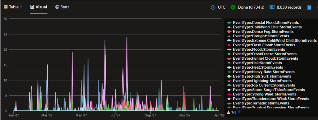
Just running the make-series operator is not enough to display the timeline chart, we also need to run the “mv-expand” operator so that it can expand into individual rows the initial results that are provided by the “make-series” operator.
let startTime1 = datetime('01-01-2007');
let endTime1 = datetime('01-01-2008');
let binSize = 1d;
StormEvents
| where StartTime between (startTime1 .. endTime1 )
| where State =~ 'Florida'
| make-series StormEvents = count() default = 0 on StartTime from startTime1 to endTime1 step binSize by EventType
| mv-expand StartTime to typeof(datetime ), StormEvents to typeof(int)
| render timechart
Time Series Functions
| Function | Explanation | Example |
|---|---|---|
| series_fir() | Applies a Finite Impulse Response (FIR) filter on a series. | range timeValues from bin( now(), 1h) – 23h to bin( now(), 1h) step 1h | summarize timeValues = make_list(timeValues) | project values = dynamic( [0, 0, 5, 10, 15, 20, 25, 100, 25, 20, 15, 10, 5, 0, 0] ), timeValues | extend MovingAverage3Hour = series_fir(values, dynamic([1,1,1])) | extend MovingAverage3HourCentered = series_fir(values, dynamic([1,1,1]), true, true) | render timechart |
| series_moving_avg_fl() | Applies a moving average filter on a series. | range timeValues from bin( now(), 1h) – 23h to bin( now(), 1h) step 1h | summarize timeValues = make_list(timeValues) | project values = dynamic( [0, 0, 5, 10, 15, 20, 25, 100, 25, 20, 15, 10, 5, 0, 0] ), timeValues | extend MovingAverage3Hour = series_moving_avg_fl(values, 3, true) | render timechart |
| series_fit_line() | Applies linear regression on a series, returning multiple columns. | demo_series3 | extend (RSquare, Slope, Variance, RVariance, Interception, LineFit) = series_fit_line(num) | render timechart |
| series_fit_2lines() | Applies a two-segmented linear regression on a series, returning multiple columns. | demo_series2 | extend series_fit_line(y), series_fit_2lines(y) | render linechart with (xcolumn = x) |
| series_decompose() | Applies a decomposition transformation on a series. | let startTime = toscalar(demo_make_series1 | summarize min(TimeStamp)); let endTime = toscalar(demo_make_series1 | summarize max(TimeStamp)); let binSize = 1h; demo_make_series1 | where Country == “United States” | make-series RequestCount = count() default = 0 on TimeStamp from startTime to endTime step binSize by Country | extend series_decompose(RequestCount, -1, ‘LineFit’) | render timechart |
| series_decompose_anomalies() | The function takes an expression containing a series (dynamic numerical array) as input, and extracts anomalous points with scores.Anomaly Detection is based on series decomposition. | let startTime = toscalar(demo_make_series1 | summarize min(TimeStamp)); let endTime = toscalar(demo_make_series1 | summarize max(TimeStamp)); let binSize = 1h; demo_make_series1 | where Country in (“United States”, “Greece”, “France”) | make-series RequestCount = count() default = 0 on TimeStamp from startTime to endTime step binSize by Country | extend anomalies = series_decompose_anomalies(RequestCount) | render anomalychart with (anomalycolumns = anomalies) |
| series_decompose_forecast() | Forecast based on series decomposition. Takes an expression containing a series (dynamic numerical array) as input, and predicts the values of the last trailing points. | let ts=range t from 1 to 24*7*4 step 1 // generate 4 weeks of hourly data | extend Timestamp = datetime(2018-03-01 05:00) + 1h * t | extend y = 2*rand() + iff((t/24)%7>=5, 5.0, 15.0) – (((t%24)/10)*((t%24)/10)) + t/72.0 // generate a series with weekly seasonality and ongoing trend | extend y=iff(t==150 or t==200 or t==780, y-8.0, y) // add some dip outliers | extend y=iff(t==300 or t==400 or t==600, y+8.0, y) // add some spike outliers | make-series y=max(y) on Timestamp from datetime(2018-03-01 05:00) to datetime(2018-03-01 05:00)+24*7*5h step 1h; // create a time series of 5 weeks (last week is empty) ts | extend y_forcasted = series_decompose_forecast(y, 24*7) // forecast a week forward | render timechart |
| series_multiply() | Calculates the element-wise multiplication of two numeric series inputs. | range x from 1 to 5 step 1 | extend y = x * 2 | extend multiply = series_multiply(pack_array(x), pack_array(y)) |
| series_divide() | Calculates the element-wise division of two numeric series inputs. | range x from 1 to 5 step 1 | extend y = x * 2 | extend divide = series_divide(pack_array(x), pack_array(y)) |
| series_greater() | Calculates the element-wise greater (>) logic operation of two numeric series inputs. | print array1 = dynamic([1,3,5]), array2 = dynamic([5,3,1]) | extend greater = series_greater(array1, array2) |
| series_acos() | Calculates the element-wise arccosine function of the numeric series input. | print array1 = dynamic([-1,0,1]) | extend arccosine = series_acos(array1) |
Plugins
Invokes a service-side query extension (plugin).
The evaluate operator is a tabular operator that allows you to invoke query language extensions known as plugins. Unlike other language constructs, plugins can be enabled or disabled. Plugins aren’t “bound” by the relational nature of the language. In other words, they may not have a predefined, statically determined, output schema. One of the plugins is the pivot plugin, which is covered in one of the tables above, and there are many more like some of the ones used in Machine Learning, such as the “autocluster” and “basket” plugins.
Check more about Plugins at the Microsoft Documentation page: https://learn.microsoft.com/en-us/azure/data-explorer/kusto/query/evaluateoperator
Geospatial Analysis
| Function | Explanation | Example |
|---|---|---|
| geo_point_in_circle() | Calculates whether the geospatial coordinates are inside a circle on Earth. | StormEvents | where isnotempty(BeginLat) and isnotempty(BeginLon) | project BeginLon, BeginLat, EventType | where geo_point_in_circle(BeginLon, BeginLat,-82.78, 27.97, 10000) | render scatterchart with (kind = map) |
| geo_distance_point_to_line() | Calculates the shortest distance in meters between a coordinate and a line or multiline on Earth. | let southCoast = dynamic({“type”:”LineString”,”coordinates”:[[-97.185,25.997],[-97.580,26.961],[-97.119,27.955],[-94.042,29.726],[-92.988,29.821],[-89.187,29.113],[-89.384,30.315],[-87.583,30.221],[-86.484,30.429],[-85.122,29.688],[-84.001,30.145],[-82.661,28.806],[-82.814,28.033],[-82.177,26.529],[-80.991,25.204]]}); StormEvents | project BeginLon, BeginLat, EventType | where geo_distance_point_to_line(BeginLon, BeginLat, southCoast) < 5000 | render scatterchart with (kind = map) |
| geo_distance_2points() | Calculates the shortest distance in meters between two geospatial coordinates on Earth. | print distance_in_meters = geo_distance_2points(-122.407628, 47.578557, -118.275287, 34.019056) |
References
- Microsoft KQL Documentation: https://learn.microsoft.com/en-us/azure/data-explorer/kusto/query/
- Kusto render operator: https://learn.microsoft.com/en-us/azure/data-explorer/kusto/query/renderoperator?pivots=azuredataexplorer
- Contoso Sales at Azure Data Explorer: https://dataexplorer.azure.com/clusters/help/databases/ContosoSales
- Azure Test Logs to practice with real data: https://portal.azure.com/#view/Microsoft_OperationsManagementSuite_Workspace/LogsDemo.ReactView/analytics/undefined
- Udemy course “Kusto Query Language (KQL) – Part 1” by Randy Minder: https://www.udemy.com/course/kusto-query-language-kql-part-1/learn/lecture/33214606#overview
- Udemy course “Kusto Query Language (KQL) – Part 2” by Randy Minder: https://www.udemy.com/course/kusto-query-language-kql-part-2/learn/lecture/38977688#overview
- Kusto Detective Agency (for practice) https://detective.kusto.io/
- Microsoft’s Github KQL Documentation: https://github.com/microsoft/Kusto-Query-Language/tree/master