As a Data Science Masters student, I’m constantly working with mathematical concepts. From the calculus behind gradient descent to the linear algebra that powers PCA, math is the bedrock of everything we do. Recently, while tackling some homework, I stumbled upon a Python library that completely changed how I approach these problems: SymPy.
Before we jump in, it’s worth noting that this post is a high-level tour to get you up and running fast. For a complete, in-depth exploration of every function and feature, your ultimate resource is the official SymPy documentation. It’s incredibly comprehensive, with detailed tutorials and API references. I highly recommend bookmarking it for when you’re ready to dive deeper!
I was so fascinated by its power that I decided to put together this quick guide. Think of it as a cheat sheet for getting started with SymPy, so you can spend less time scribbling algebra on paper and more time coding.
Table of Contents
- What is SymPy?
- Getting Started: The Basics
- Core Functions: Your Mathematical Toolkit
- The Visual Magic: Plotting with SymPy
- The Plot Function
- Why This Matters for Data Science
What is SymPy?
Most Python libraries for math, like NumPy, are numerical. They work with numbers (like 3.14159). SymPy is different. It’s a library for symbolic mathematics. It works with symbols and expressions, just like you would in an algebra or calculus class. This means it can give you the exact, analytical answer, not just a numerical approximation.
Getting Started: The Basics
First things first, let’s install it and import it. I like to use init_printing() to make the output look clean and mathematical (it renders in LaTeX if you’re in a Jupyter Notebook).
# Installation in your terminal
# pip install sympy

# In your Python script or notebook
import sympy as sp

# This makes the output look pretty
sp.init_printing(use_unicode=True)
The most fundamental concept in SymPy is the Symbol. You must declare any symbolic variables you want to use.
# Declare a single symbol
x = sp.symbols('x')

# Declare multiple symbols at once
y, z = sp.symbols('y z')

# Now we can create a symbolic expression
expr = x**2 + 2*y + z
expr
Output:
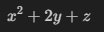
See? It’s not a number; it’s the actual mathematical expression!
Core Functions: Your Mathematical Toolkit
Let’s dive into the core functions that you’ll use most often.
1. Algebraic Manipulation: expand(), factor(), and simplify()
These are your best friends for cleaning up complex expressions.
- expand(): Multiplies everything out.
- factor(): Pulls out common factors (the opposite of expand).
- simplify(): Tries various techniques to simplify an expression into its “nicest” form.
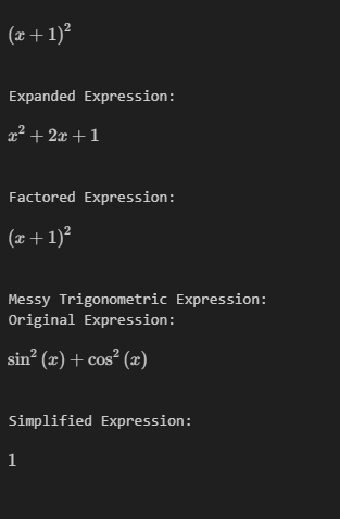
# Let's create an expression
expr = (x + 1)**2
print("Original Expression:")
display(expr)

# Expand it
expanded_expr = sp.expand(expr)
print("\nExpanded Expression:")
display(expanded_expr)

# Factor it back
factored_expr = sp.factor(expanded_expr)
print("\nFactored Expression:")
display(factored_expr)

# A more complex example for simplify()
messy_expr = sp.sin(x)**2 + sp.cos(x)**2
print("\nMessy Trigonometric Expression:")
display(messy_expr)

simplified_expr = sp.simplify(messy_expr)
print("\nSimplified Expression:")
display(simplified_expr)
Output:
2. Substitution: subs()
This is incredibly useful for evaluating an expression at a certain point.
expr = x**2 + 3*x + 5
# Substitute x with a number
result = expr.subs(x, 2)
print(f"Expression evaluated at x=2: {result}") # Output: 15
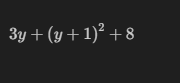
# Substitute x with another expression
new_expr = expr.subs(x, y + 1)
display(new_expr)
Output:
3. Calculus: The Data Scientist’s Bread and Butter
This is where SymPy truly shines for machine learning folks. Understanding the derivatives and integrals that define your optimization algorithms is key.
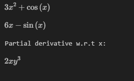
- diff() for Derivatives: Find the derivative of an expression. You can also compute partial derivatives.
# Our expression
expr = x**3 + sp.sin(x)

# First derivative with respect to x
derivative = sp.diff(expr, x)
display(derivative)

# Second derivative
second_derivative = sp.diff(expr, x, 2)
display(second_derivative)

# Partial derivatives
expr_xy = x**2 * y**3
partial_deriv_x = sp.diff(expr_xy, x)
print("Partial derivative w.r.t x:")
display(partial_deriv_x)
Output:
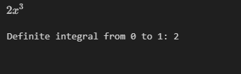
- integrate() for Integrals: Compute both indefinite and definite integrals.
# Indefinite integral (antiderivative)
indef_integral = sp.integrate(6*x**2, x)
display(indef_integral)

# Definite integral from 0 to 1
def_integral = sp.integrate(6*x**2, (x, 0, 1))
print(f"Definite integral from 0 to 1: {def_integral}")
Output:
4. Solving Equations: solveset()
Need to find the roots of an equation? solveset() is the modern, recommended way to do it.
# We want to solve x**2 - 4 = 0
equation = sp.Eq(x**2, 4)
solutions = sp.solveset(equation, x)
display(solutions)
Output:

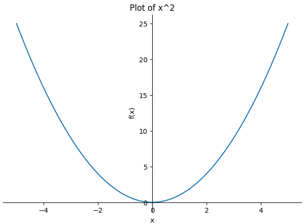
The Visual Magic: Plotting with SymPy
Yes, you can even create charts directly with SymPy! While libraries like Matplotlib or Seaborn are more powerful for data visualization, SymPy’s plotting is perfect for quickly visualizing a symbolic function.
from sympy.plotting import plot, plot3d

# A simple 2D plot
p1 = plot(x**2, (x, -5, 5), title="Plot of x^2", show=False)

# Plotting multiple functions
p2 = plot(sp.sin(x), sp.cos(x), (x, -2*sp.pi, 2*sp.pi), show=False)
p1.show()
p2.show()
This will generate two plots:
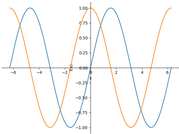
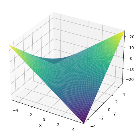
You can even do 3D plots with ease!
# A 3D plot
plot3d(x * y, (x, -5, 5), (y, -5, 5))
3D Plot Output:
The Plot Function
Required Parameters
- Expression: The SymPy expression to plot
- Range: Tuple (x, xmin, xmax) specifying:
- x: Symbol variable for the expression
- xmin, xmax: Start and end values for the x-axis
Optional Parameters
Display Control
- show (bool, default=True): Whether to display the plot immediately
- title (str): Title of the plot
- xlabel, ylabel (str): Axis labels
- xlim, ylim (tuple): Axis limits as (min, max)
Style Parameters
- line_color (str or RGB tuple): Color of the line (e.g., ‘red’, ‘#FF0000’)
- line_width (float, default=1.0): Width of the plotted line
- adaptive (bool, default=True): Whether to use adaptive sampling
- depth (int): For adaptive sampling, level of recursion
- nb_of_points (int, default=100): Number of points when not using adaptive sampling
Legend and Grid
- legend (bool, default=False): Whether to show a legend
- grid (bool, default=False): Whether to show a grid
- annotations (list): List of annotation objects to add
Formatting
- xscale, yscale (str): Scale type (‘linear’, ‘log’, etc.)
- axis_center (tuple or bool): Position of axis crossing
- aspect_ratio (str or tuple): Control aspect ratio
- size (tuple): Size of the figure as (width, height) in pixels
Backend Options
- backend (str, default=’matplotlib’): Plotting backend to use
- backend_options (dict): Options to pass to the backend
Why This Matters for Data Science
SymPy isn’t just a toy. It’s a serious tool that can:
- Verify analytical solutions: Double-check the derivatives you calculated for your custom loss function.
- Understand algorithms: See the exact form of a complex equation before you try to implement it numerically.
- Simplify complex models: Use simplify() to see if a messy-looking model can be reduced to something more elegant.
This has been a whirlwind tour, but I hope it serves as a great starting point and a handy reference for your future projects.
Happy calculating!